Example using a subset of data
Introduction
Here you can find a tutorial for calculating receiver functions and time-to-depth calculation for a given subset of seismic waveform data from the EASI seismic network. Note that this is only a small sample of all the available data and its only purpose is to show the functionality of the codes. The example dataset is available in the following link.
Here we start from continuous data cut around the arrival times of selected teleseismic events and apply a systematic processing routine (see Figure 1 for details on the steps we follow).
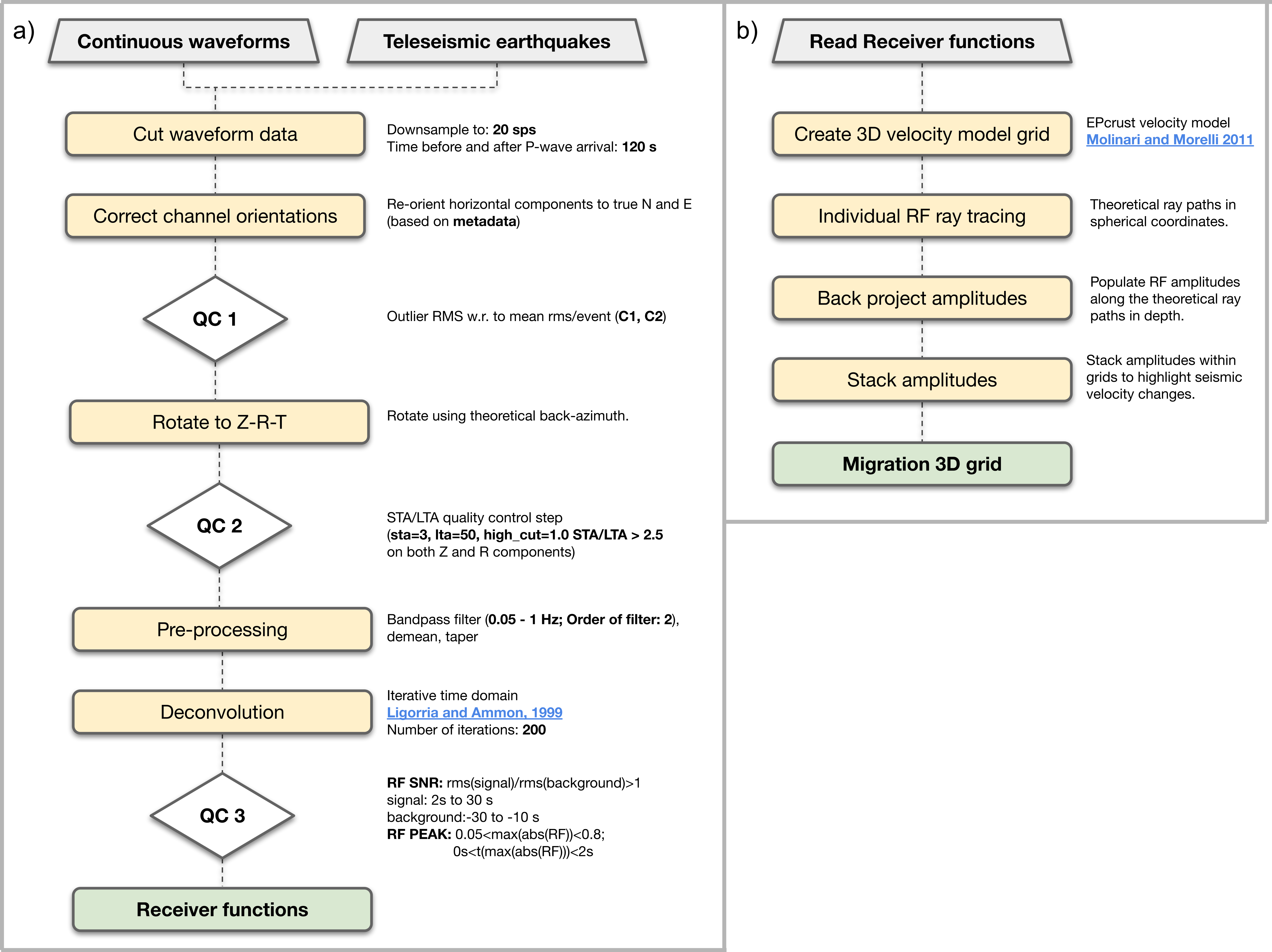
Processing steps for Receiver Function and time-to-depth migration calculations within rfmpy.
Download example dataset
First we need to download the seismic waveform data from a ZENODO repository in our local computer.
Create a directory to store the waveform data:
$ mkdir ~/Desktop/data_sample
Download the data sample from ZENODO in that directory along with two files (plot_EASI.sh,vk.cpt) that we will need later:
$ wget https://zenodo.org/record/7292588/files/seismic_data.tar.xz -P ~/Desktop/data_sample/
[2022-09-27 15:56:54]  https://zenodo.org/record/7292588/files/seismic_data.tar.xz
Resolving zenodo.org (zenodo.org)... 188.184.117.155
Connecting to zenodo.org (zenodo.org)|188.184.117.155|:443... connected.
HTTP request sent, awaiting response... 200 OK
Length: 141181064 (135M) [application/octet-stream]
Saving to: ‘~/Desktop/data_sample/seismic_data.tar.xz’
seismic_data.tar.xz.2             100%[==========================================================>] 134.64M  8.43MB/s    in 13s
[2022-09-27 15:57:08] (10.2 MB/s) - ‘~/Desktop/data_sample/seismic_data.tar.xz’ saved [141181064/141181064]
$ wget https://zenodo.org/record/7292588/files/plot_EASI.sh -P ~/Desktop/data_sample/
$ wget https://zenodo.org/record/7292588/files/vik.cpt -P ~/Desktop/data_sample/
Resolving zenodo.org (zenodo.org)... 188.184.117.155
Connecting to zenodo.org (zenodo.org)|188.184.117.155|:443... connected.
HTTP request sent, awaiting response... 200 OK
Length: 602 [application/octet-stream]
Saving to: ‘~/Desktop/data_sample/plot_EASI.sh.1’
Saving to: ‘~/Desktop/data_sample/vik.cpt.1’
plot_EASI.sh.1      100%[===================>]     602  --.-KB/s    in 0s
vik.cpt.1           100%[===================>]   9.86K  --.-KB/s    in 0s
Extract files from the tar file we just downloaded:
$ tar -xf ~/Desktop/data_sample/seismic_data.tar.xz --directory ~/Desktop/data_sample
Create a directory to store RFs:
$ mkdir ~/Desktop/data_sample/RF
$ mkdir ~/Desktop/data_sample/TRF
Calculate receiver functions
Run the following, code snippet from the repository’s top folder to compute receiver functions.
import rfmpy.core.RF_Main as RF
from obspy import read_inventory, read_events, UTCDateTime as UTC
import os
import time

# Define working directory
work_dir = os.getcwd()

# Path in which waveforms are stored
path_wavs = ['/home/' + work_dir.split('/')[2] + '/Desktop/data_sample/EASI/data/']

# Define path to store RFs
path_out_RF = '/home/' + work_dir.split('/')[2] + '/Desktop/data_sample/'

# Start a timer to keep a track how long the calculations take
t_beg = time.time()

# Path for StationXML files
path_meta = work_dir + '/data/metadata/'
try:
    print('>>> Reading inventory...')
    inv = read_inventory(path_meta + '/*.xml')
    print('>>> Read inventory...')
except Exception as e:
    raise type(e)('>>> Move to the top directory of the repository!')

# =================================================== #
# Define parameters for calculating receiver functions
# Define sta/lta parameters
sta_lta_qc_parameters = {'sta': 3, 'lta': 50, 'high_cut': 1.0, 'threshold': 2.5}

# Define pre-processing parameters
pre_processing_parameters = {'low_cut': 0.05, 'high_cut': 1.0, 'order': 2,
                             't_before': 40, 't_after': 60}
for path_wav in path_wavs:
    print(path_wav)
    RF.calculate_rf(path_ev=path_wav, path_out=path_out_RF, inventory=inv, iterations=200,
                    ds=30, c1=10, c2=10, sta_lta_qc=sta_lta_qc_parameters,
                    pre_processing=pre_processing_parameters, max_frequency=1, save=True, plot=False)
# ==================================================== #
t_end = time.time()
total_time = t_end - t_beg
print('It took ' + str(round(total_time)/60) + ' minutes in total.')
[2022-09-27 15:58:01] >>> Reading inventory...
>>> Read inventory...
/home//Desktop/data_sample/EASI/data/
Calculating RF for event in: /home//Desktop/data_sample/EASI/data/P_2014.363.09.29.37
...
>>> Station: XT.AAE50 - Failed on QC 2.
[2022-09-27 16:57:08] It took 20 minutes in total.
This created 273 RF files in SAC format…
Calculate time-to-depth migration
Now to compute time-to-depth migration for these RF traces we use the following code snippet.
import rfmpy.core.migration_sphr as rf_mig
import rfmpy.utils.migration_plots_spher as plot_migration_sphr
import os
import time

# Start a timer to keep a track how long the calculations take
t_beg = time.time()

# Define working directory
work_dir = os.getcwd()

# Define path to RFs
path = '/home/' + work_dir.split('/')[2] + '/Desktop/data_sample/RF/'

# Read station coordinates from the rfs (sac files) in a pandas dataframe
sta = rf_mig.read_stations_from_sac(path2rfs=path)

# Read RFs
stream = rf_mig.read_traces_sphr(path2rfs=path, sta=sta)

# =================================================== #
# Define MIGRATION parameters
# Ray-tracing parameters
inc = 0.25
zmax = 100
# Determine study area (x -> perpendicular to the profile)
minx = 0.0
maxx = 30.0
pasx = 0.05
miny = 30.0
maxy = 60.0
pasy = 0.05
minz = -5
# maxz needs to be >= zmax
maxz = 100
pasz = 0.5
# Pass all the migration parameters in a dictionary to use them in functions called below
m_params = {'minx': minx, 'maxx': maxx,
            'pasx': pasx, 'pasy': pasy, 'miny': miny, 'maxy': maxy,
            'minz': minz, 'maxz': maxz, 'pasz': pasz, 'inc': inc, 'zmax': zmax}


# Ray tracing
# Pick one of the two velocity models
# 'EPcrust' or 'iasp91'
# We use EPcrust velocity model here...
stream_ray_trace = rf_mig.tracing_3D_sphr(stream=stream, migration_param_dict=m_params,
                                          velocity_model='EPcrust')

# Write piercing points in a file
plot_migration_sphr.write_files_4_piercing_points_and_raypaths(stream_ray_trace, sta, piercing_depth=35, plot=True)
# Migration
mObs = rf_mig.ccpm_3d(stream_ray_trace, m_params, output_file="/home/" + work_dir.split('/')[2] + "/Desktop/data_sample/epcrust", phase="PS")
total_time = time.time() - t_beg
print('Time-to-depth migration took ' + str(round(total_time)/60) + ' minutes in total.')
|-----------------------------------------------|
| Reading receiver functions...                 |
| Reading trace 0 of 273
...
| 273 of 273
| End of 3D ray tracing...                      |
|-----------------------------------------------|
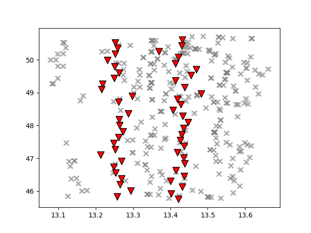
Map showing the piercing points (gray crosses) at 35 km depth computed for each seismic station (inverted red triangles) using the EPcrust velocity model (Molinari and Morelli, 2011).
|-----------------------------------------------|
| Start of common conversion point stacking...  |
| 1 of 273
...
| 273 of 273
| End of common conversion point stacking...    |
|-----------------------------------------------|
Time-to-depth migration took 0.7 minutes in total.
This provides us with a 3D grid (epcrust.npy) of stacked migrated RF amplitudes.
Plot migrated cross-sections
We will use this 3D grid to plot the cross-section using GMT6. Before we do this, we need to create the cross-section
import rfmpy.core.migration_sphr as rf_mig
import rfmpy.utils.migration_plots_spher as plot_migration_sphr
import numpy as np
import os
import matplotlib.pyplot as plt
from obspy.geodetics import degrees2kilometers, kilometers2degrees

path2grid = '/home/' + work_dir.split('/')[2] + '/Desktop/data_sample/'

# Read the 3D grid (epcrust.npy) of stacked migrated RF amplitudes.
with open(path2grid + 'epcrust.npy', 'rb') as f:
    mObs_ep = np.load(f)

profile = np.array([[13.35, 50.6], [13.35, 45.6]])
profile_name = 'EASI'
G2_, sta, xx, zz = plot_migration_sphr.create_2d_profile(mObs_ep, m_params, profile, sta, swath=37.5, plot=True)
mObs = rf_mig.ccp_smooth(G2_, m_params)
mObs = rf_mig.ccpFilter(mObs)


# File for GMT plot
for i, x in enumerate(xx):
    for j, z in enumerate(zz):
        print(kilometers2degrees(x), z, mObs[i,j])
        with open(path2grid + profile_name + '.txt', 'a') as of:
            of.write('{} {} {} \n'.
                     format(kilometers2degrees(x), z, mObs[i, j]))
Using the following commands we can create the cross-section using the GMT6 code we downloaded.
$ cd ~/Desktop/data_sample/
$ conda deactivate
$ conda activate gmt6
$ bash plot_EASI.sh
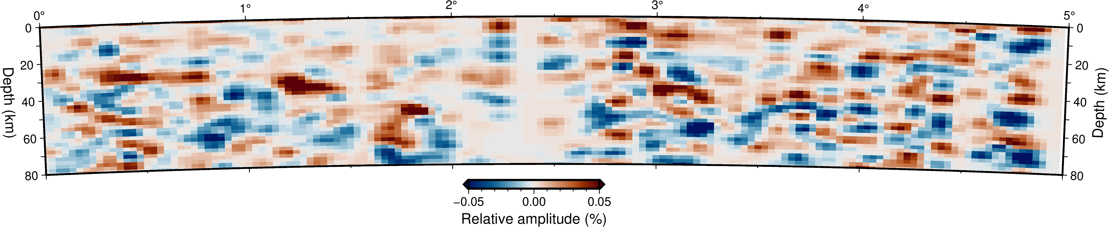
Migrated receiver-function cross-sections along the EASI seismic network.